An Ordinal Classification Metric: Closeness Evaluation Measure

17 May 2024 in Blog

Introduce an evaluation metric for the ordinal classification task.

Streamlit: Demo App | Code: Github | CEM Paper: ACL

Introduction Permalink

Ordinal classification is a type of classification task whose predicted classes (or categories) have a specific ordering. This implies misclassifying a class pair should be penalized differently and proportionally, with respect to their semantic order and class distribution in a dataset. Existing evaluation metrics are shown failed to capture certain aspects of this task, that it calls for the employment of a new metric, namely Closeness Evaluation Measure ( CEM$CEM$).

For example,

• precision/recall ignores the ordering among classes.
• mean average error/mean squared error assumes a predefined interval between classes, subject to their numeric encoding.
• ranking measures indeed capture the relative ranking in terms of relevancy, but lack of emphasis on identifying the correct class.

CEM$CEM$ employs the idea of informational closeness: the less LIKELY there is data point between a class pair, the closer they are. As a result, a model that misclassifies informational-close classes should be penalized lesser than those informational-distant. It has been mathematically proven this measure attains the desired properties that addresses the foregoing shortcomings, which to be discussed shortly after.

This post is divided as follows (for a more interactive experience, checkout the streamlit demo):

• Information Closeness
• Closeness Evaluation Measure
• Metric Properties
• An Example Usecase

Information Closeness Permalink

Let’s say we have two journals F$F$ and S$S$ (mockup data in Fig. 1.) with two very distinct natures of reviewing research paper submissions. Reviewers at journal F$F$ are very cautious and it’s rare to see they review a paper as reject or accept. Journal S$S$, on the other hand, tends to take a clear stance on the paper’s acceptance/rejection status.

Given that, weak reject vs. weak accept in the context of S$S$ are informational close because they are closer assessment, while F$F$ treating them as two far ends of the grading scales due to the fact this is a strong disagreement between reviewers in the context of F$F$. Put it differently, two classes a$a$ and b$b$ are informationally close if the probability of finding data points between the two is low.

More formally, given a set of ordinal classes C=\{c_1, ..., c_m\}$C=\{c_1, ..., c_m\}$ and amount of data points assigned to each class \{n_1, ..., n_m\}$\{n_1, ..., n_m\}$ with N=\Sigma_{i=1}^{m} n_i$N=\Sigma_{i=1}^{m} n_i$, the informational closeness of any class pair IC(c_i, c_j)$IC(c_i, c_j)$ is the inverse -log(.)$-log(.)$ of the probability of data points assigned to classes in between (\frac{n_i}{2} + \Sigma_{k=i+1}^{j} n_k)/N$(\frac{n_i}{2} + \Sigma_{k=i+1}^{j} n_k)/N$.

Put it all together, we have

IC(c_i, c_j) = -log(\frac{\frac{n_i}{2} + \Sigma_{k=i+1}^{j} n_k}{N})

$IC(c_i, c_j) = -log(\frac{\frac{n_i}{2} + \Sigma_{k=i+1}^{j} n_k}{N})$

To be clear,

IC(c_1, c_3) = -log(\frac{n_1/2 + n_2 + n_3}{N})

$IC(c_1, c_3) = -log(\frac{n_1/2 + n_2 + n_3}{N})$

IC(c_3, c_1) = -log(\frac{n_3/2 + n_2 + n_1}{N})

$IC(c_3, c_1) = -log(\frac{n_3/2 + n_2 + n_1}{N})$

IC(c_1, c_1) = -log(\frac{n_1/2}{N})

$IC(c_1, c_1) = -log(\frac{n_1/2}{N})$

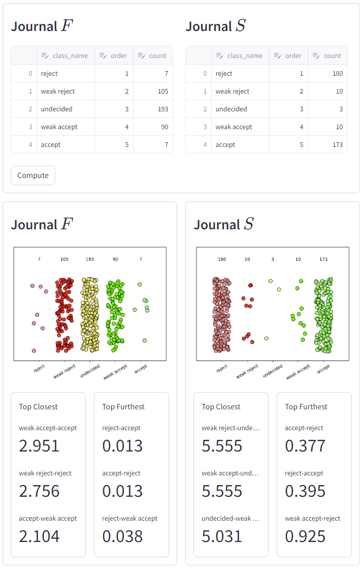
Fig. 1. Two journals F$F$ and S$S$ with two very distinct natures of reviewing research paper submissions.

In the above charts, for each journal, we computed IC$IC$ for all class combinations and show the top closest and furthest pairs. As expected, both journals agree that reject vs. accept is the furthest pair. Journal S$S$ treats those on the border: weakly reject, undecided, weakly accept as closest pairs, given there are small amount of data points between them.

Note that, IC$IC$ is not symmetrical, hence IC(c_i, c_j) \neq IC(c_j, c_i)$IC(c_i, c_j) \neq IC(c_j, c_i)$. Also for the ease of readability, we scale the computed value by a constant of 1/log(2)$1/log(2)$.

Closeness Evaluation Measure Permalink

Next question: How to formulate the idea of informational closeness to an usable evaluation metric for ordinal classification task?

It’s simple. Assume you have an ordinal classification dataset whose each data point labelled an ordinal class. Firstly, you compute the IC$IC$ for classes in the dataset; this quantity translates to the reward for making an ordinal step from one class to another which are distributionally closer. Secondly, assume you have a candidate Machine Learning model has been trained on such dataset and ready to evaluate. For each data point, we favour prediction whose class is close to the groundtruth; an accurate class matching results to a point 1$1$, while the lesser earning a lesser point. Doing the same for all predictions, we obtain the overall performance measure, i.e. CEM$CEM$. The highest achievable score for CEM$CEM$ is 1$1$, that is, the higher the better.

More formally, given a dataset D$D$, a groundtruth label mapping, g: D \rightarrow C$g: D \rightarrow C$, an ML model m: D \rightarrow C$m: D \rightarrow C$, the closeness evaluation measure of such model CEM(m, g)$CEM(m, g)$ is the summation of IC$IC$ between predicted class and groundtruth, normalized by IC$IC$ of the groundtruth itself, IC[m(d), g(d)] / IC[g(d), g(d)]$IC[m(d), g(d)] / IC[g(d), g(d)]$ across all data points (\Sigma_{d \in D}$\Sigma_{d \in D}$).

Put together, we have

CEM(m, g) = \frac{\Sigma_{d \in D} IC[m(d), g(d)]} {\Sigma_{d \in D} IC[g(d), g(d)]}

$CEM(m, g) = \frac{\Sigma_{d \in D} IC[m(d), g(d)]} {\Sigma_{d \in D} IC[g(d), g(d)]}$

Metric Properties Permalink

CEM$CEM$ has been proven to satisfy three mathematical properties that address the shortcomings of other metrics. That is, the metrics take into account of ordering information, does not assume a predefined interval between classes, and reward the highest score for identifying the correct class.

Below are subsections elaborating the properties. Each property to be accompanied by a pair of exampled datasets, whose groundtruth and prediction are depicted in the x-axis and coloring, respectively. This to illustrate the intuition behind each property, and in order to read the charts properly, do pay attention to Ordinal Invariance section.

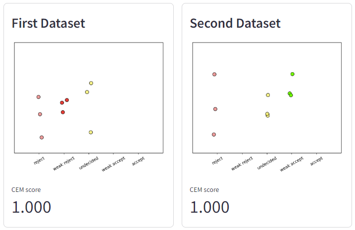
Ordinal Invariance Permalink

First Dataset is a journal paper review dataset with 9$9$ data points. The x-axis’ ticks depict their true classes: 3$3$ rejects, 3$3$ weak rejects, 3$3$ undecideds and 0$0$ for the other two classes. The coloring of the circles ( pink, red, yellow, dark green, light green), depicts the data points’ predictions. In this data set, the 9$9$ predictions are exact matches to their true classes.

Second Dataset is similar with 100 \%$100 \%$ match for other set of classes: 3$3$ rejects, 3$3$ undecideds, 3$3$ weak accepts. Its mere difference is that its groundtruth shifted their value to strictly higher-order classes.

Therefore, Ordinal Invariance states that the metric value should remain the same if a dataset have its model output and groundtruth shift their value in a strictly higher-order classes.

Fig. 2. Ordinal Invariance.

Monotonicity Permalink

Monotonicity states that, changing the model output closer to the groundtruth should result in a metric increase.

Indeed, First Dataset have one weak accept point misclassified as undecided. Second Dataset should perform worse because the very same data point is misclassified to a further class, i.e. weak reject.

Fig. 3. Monotonicity.

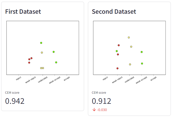
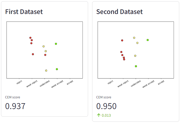
Imbalance Permalink

Imbalance states that, a classification error in a small class should have lesser impact - or receive higher reward - in comparison to the same mistake in a frequent class.

First Dataset misclassifies a data point from a frequent class, weak reject, should have lower metric value than Second Dataset that misclassifies a data point from a small class, i.e. weak accept.

There is an inconsistency in my interpretation and the original paper. I have contacted the author for advice regarding this discrepancy. Raised Issue

Fig. 4. Imbalance.

An Example Usecase Permalink

Let’s put CEM$CEM$ into a test!

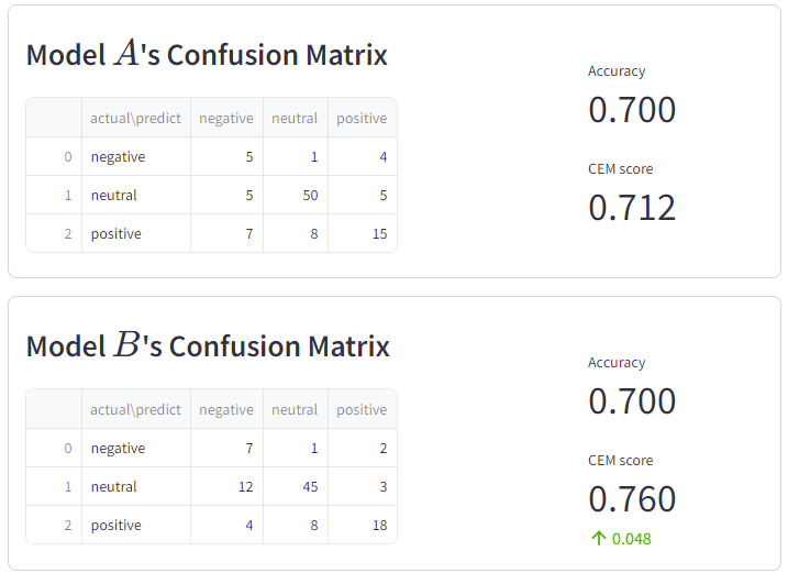
Given a dataset, we have the confusion matrix for two model A$A$ and B$B$ as followings. From accuracy metric standpoint, both models are on par. CEM$CEM$ said otherwise and highlights that model B$B$ should be the better performer.

It is indeed a true evaluation, in view that:

• Model A$A$ makes more mistakes between distant classes: positive-negative (7+4 > 4+2$7+4 > 4+2$).
• Model A$A$ makes more mistakes in positive-neutral, whose population represent 90 \%$90 \%$ of the dataset, hence penalized more heavily, or precisely, earning less reward.

Fig. 5. Imbalance.

---